This is the supporting page for our paper FastDTW is approximate and Generally Slower than the Algorithm it Approximates.
Keywords: Dynamic time warping, time series analysis, similarity measures, and data mining.
Update (Jan. 25, 2021): Extended abstract accepted by 37th IEEE International Conference on Data Engineering (ICDE2021), TKDE Posters Track.
Update (Oct. 23, 2020): Accepted by IEEE Transactions on Knowledge and Data Engineering (TKDE), doi:10.1109/TKDE.2020.3033752.
@Article{Wu2020,
  author    = {Renjie Wu and Eamonn J. Keogh},
  journal   = {{IEEE} Transactions on Knowledge and Data Engineering},
  title     = {{FastDTW} is Approximate and Generally Slower Than the Algorithm it Approximates},
  year      = {2022},
  number    = {8},
  pages     = {3779--3785},
  volume    = {34},
  doi       = {10.1109/TKDE.2020.3033752},
  publisher = {Institute of Electrical and Electronics Engineers ({IEEE})},
}
Presentation at ICDE2021
Code
cDTW alone
The original cDTW code is written by Sara Alaee (my labmate) in C++. But to be fair with FastDTW (which is written in Java), we re-wrote Sara’s cDTW code in Java. Here we also provide a Python implementation.
- C++: dtwupd.h, dtwupd.cpp. Requires at least C++ 11.
- Java: DtwUpd.java. Requires at lease JDK 11.
- Python: dtwupd.py. Written in Python 3.6.
- MATLAB:
dist = dtw(A, B, radius, 'squared');Built-in function.
Java project
To compile the code, JDK 11 is required to be installed. The project is written with IntelliJ IDEA Ultimate 2019.3.
- Project: DTWPublish-v1.zip. SHA1:
d19818a89b8b4f4909a010194a225e432af44d20
This zip file ships with FastDTW-modified-1.1.0.jar, so you don’t have to download it separately.
MATLAB helpers
All MATLAB helper scripts are written with MATLAB R2018b.
- Helper scripts: Helpers-v1.zip. SHA1:
3ed45abab4a50f7e901b0e76ece75976a997df41
Pre-compiled jar file
Although it should be fine to run them with JRE 1.8 (we didn’t test it), we highly recommend you use at least JRE 11.
- Modified FastDTW: FastDTW-modified-1.1.0.jar. SHA1:
6144e3f4cd464727a7ecc89d6edf31426975e167 - Project for reproducibility: DTWPublish-v1.jar. SHA1:
f9bfcb8460a91f4b26dc6f0da2e6129214720b85
Data
Case A: Short N and Narrow W
-
UWaveGestureLibraryAlldataset to produce Fig. 1 can be found in UCR Archive1. -
DataSummary.csvto produce Fig. 2 can be downloaded from here (also from UCR Archive1).
Case B: Long N and Narrow W
The two random walks of length 24,000 is generated from MATLAB script RandomWalkGenerator.m (which can be found in section Code: MATLAB helpers). The function signature is RandomWalkGenerator(length, amount, outputDir, separateFile).
The length is the length of generated random walk, amount is number of random walks to be generated, outputDir determines where the files will be stored, and separateFile is whether generated random walks should be stored in a single file or multiple files.
For Case B, we use
RandomWalkGenerator(24000, 2, "/path/to/case-b-dir/", 1)
to generate the data. You can also get them from
- Pre-generated random walk 1 of length 24,000: case-b-1.tsv.
- Pre-generated random walk 2 of length 24,000: case-b-2.tsv.
Case C: Short N and Wide W
For Case C, we use 1,000 random walks of length 450 to represent random electrical power demand. In Fig. 4, we use
RandomWalkGenerator(450, 1000, "/path/to/case-c-dir/", 0)
to generate the data. The pre-generated data.tsv can be found below.
- Pre-generated
data.csv: case-c-data.tsv.
Case D: Long N and Wide W
The artificial “Fall over anytime within L seconds of hearing the beep” dataset is generated from MATLAB script GenerateSyntheticFallsPairs.m (which can be found in section Code: MATLAB helpers). The function signature is GenerateSyntheticFallsPairs(outputPath, startL, endL).
The outputPath folder stores generated two tsv files. startL and endL determine the range of L. In Fig. 6, we use
GenerateSyntheticFallsPairs("/path/to/case-d-dir/", 0, 10)
to generate the data. They can also be downloaded below.
- Pre-generated
FallAs_0to10.tsv: FallAs_0to10.tsv. - Pre-gererated
FallBs_0to10.tsv: FallBs_0to10.tsv.
When does FastDTW fail to Approximate Well?
The three time series A, B and C used in Table. 2 can be generated via MATLAB script FastDTWFailDataset.m (which can be found in section Code: MATLAB helpers). The function signature is FastDTWFailDataset(outputDir).
The parameter outputDir determines where the file data.tsv will be written into. You can also download pre-generated data.tsv below.
- Pre-generated
data.tsv: fastdtw-fails-data.tsv.
Modification in FastDTW’s code
The original Java implementation used in Stan and Philip’s paper2 can be downloaded from here: FastDTW-1.1.0.zip. Their original project page is here.
Since the datasets from UCR Archive1 are stored in tsv format, we used the code snippet from Roberto Maestre3 to construct FastDTW’s TimeSeries object from the pure double array in tsv files.
A new constructor of TimeSeries object is added into FastDTW’s com/timeseries/TimeSeries.java:
/**
 * Ad-hoc constructor from a double array
 * ONLY ONE FIXED COLUMN
 */
public TimeSeries(double[] x) {
    // DS to create labels and values
    AtomicInteger counter = new AtomicInteger();
    TimeSeriesPoint tsValues;

    // Only one time series
    timeReadings = new ArrayList();
    ArrayList values;

    // Each value is one incremented label
    labels = new ArrayList();
    labels.add("Time");
    labels.add("c1");

    tsArray = new ArrayList();
    for (double value : x) {
        timeReadings.add((double) counter.getAndIncrement());
        values = new ArrayList();
        values.add(value);
        tsValues = new TimeSeriesPoint(values);
        tsArray.add(tsValues);
    }
}
The pre-compiled jar file of modified FastDTW can be found in section Code: Pre-compiled jar file.
Reproduce results in the paper
In the below, we use N to refer to the length of the time series being compared, r to the radius of FastDTW, and w to the user-specified warping constraint, given as a percentage of N. We use W to refer to the natural amount of warping needed two align two random examples in a domain, also given as a percentage of N.
Case A: Short N and Narrow W
Fig. 1
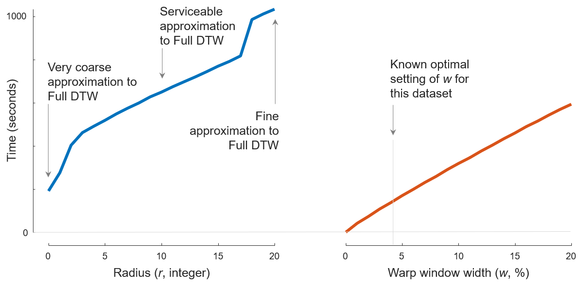
UWaveGestureLibraryAll (which requires \((896 \times 895) \div 2 = 400,960\) comparisons), for w = 0 to 20% for cDTW and for r = 0 to 20 for FastDTW. To produce Fig. 1, we first run Java code
java -cp "/path/to/DTWPublish.jar" edu.ucr.benchmark.WarpWindowPairwiseBenchmark "/path/to/UWaveGestureLibraryAll_TRAIN.tsv" 0 0 20 1 "/path/to/fastdtw-output.csv"
java -cp "/path/to/DTWPublish.jar" edu.ucr.benchmark.WarpWindowPairwiseBenchmark "/path/to/UWaveGestureLibraryAll_TRAIN.tsv" 1 0 20 1 "/path/to/cdtw-output.csv"
to measure the running time of both algorithms.
The pre-compiled DTWPublish.jar file can be found in section Code: Pre-compiled jar file; UWaveGestureLibraryAll_TRAIN.tsv can be found in section Data: Case A; /path/to/fastdtw-output.csv and /path/to/cdtw-output.csv determines where results will be written into.
Then we run MATLAB script caseAandC_TimeComparsion.m (which can be found in section Code: MATLAB helpers)
caseAandC_TimeComparsion("/path/to/fastdtw-output.csv", "/path/to/cdtw-output.csv", 0:20, 0:20)
to draw the figure.
Fig. 2
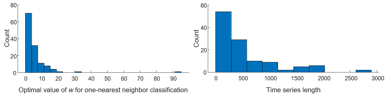
To produce Fig. 2, run MATLAB script caseA_Histogram.m (which can be found in section Code: MATLAB helpers). The function signature is caseA_Histogram(UCRArchiveDataSummryCSV). You can get DataSummary.csv in section Data: Case A.
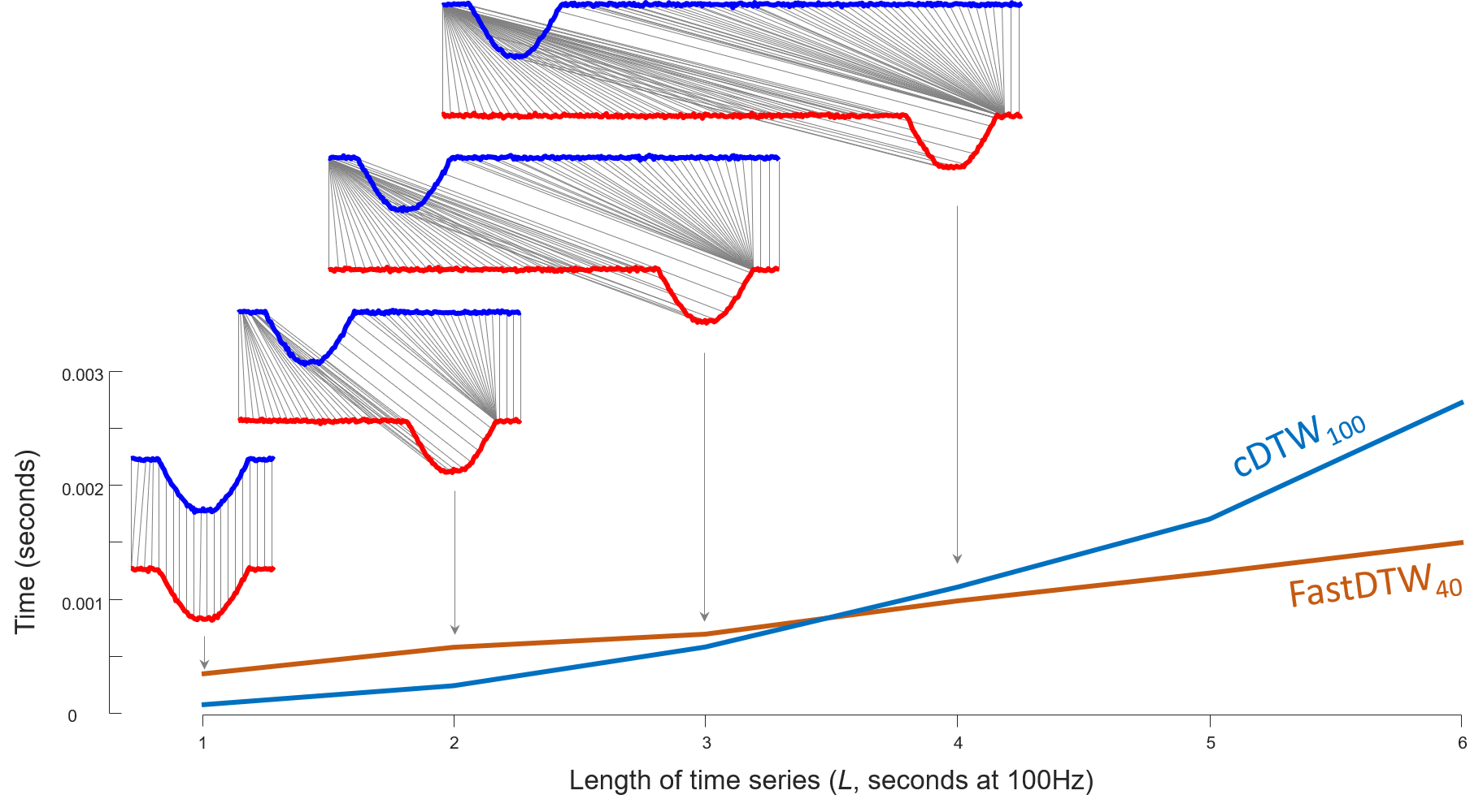
Case B: Long N and Narrow W
For Case B in the paper, we measured the running time of both algorithms on two time series of length 24,000 by reporting the average of 1,000 runs. We find that
- cDTW0.83 takes 45.6 milliseconds
- FastDTW10 takes 238.2 milliseconds
- FastDTW40 takes 350.9 milliseconds
The aforementioned average running time of both algorithms is measured by
java -cp "/path/to/DTWPublish.jar" edu.ucr.runner.PairsRunner "/path/to/1.tsv" "/path/to/2.tsv" 0.83 "/path/to/output.csv"
The pre-compiled DTWPublish.jar file can be found in section Code: Pre-compiled jar file; 1.tsv and 2.tsv can be found in section Data: Case B; /path/to/output.csv determines where results will be written into.
Case C: Short N and Wide W
Fig. 4
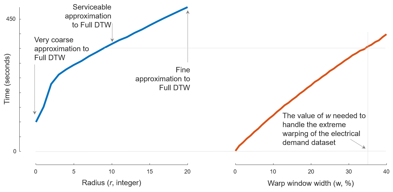
To produce Fig. 4, we first run Java code
java -cp "/path/to/DTWPublish.jar" edu.ucr.benchmark.WarpWindowPairwiseBenchmark "/path/to/data.tsv" 0 0 20 1 "/path/to/fastdtw-output.csv"
java -cp "/path/to/DTWPublish.jar" edu.ucr.benchmark.WarpWindowPairwiseBenchmark "/path/to/data.tsv" 1 0 40 1 "/path/to/cdtw-output.csv"
to measure the running time of both algorithms.
The pre-compiled DTWPublish.jar file can be found in section Code: Pre-compiled jar file; data.tsv can be found in section Data: Case C; /path/to/fastdtw-output.csv and /path/to/cdtw-output.csv determines where results will be written into.
Then we run MATLAB script caseAandC_TimeComparsion.m (which can be found in section Code: MATLAB helpers)
caseAandC_TimeComparsion("/path/to/fastdtw-output.csv", "/path/to/cdtw-output.csv", 0:20, 0:40)
to draw the figure.
Case D: Long N and Wide W
Fig. 6
The running time of both algorithms in Fig. 6 is measured by
java -cp "/path/to/DTWPublish.jar" edu.ucr.runner.PairsRunner "/path/to/FallAs_0to10.tsv" "/path/to/FallBs_0to10.tsv" 100 "/path/to/output.csv"
The pre-compiled DTWPublish.jar file can be found in section Code: Pre-compiled jar file; FallAs_0to10.tsv and FallBs_0to10.tsv can be found in section Data: Case D; /path/to/output.csv determines where results will be written into.
When does FastDTW fail to Approximate Well?
Table. 2
| A | B | C | |
|---|---|---|---|
| A | 0 | 0.020 | 6.822 |
| B | 0 | 6.848 | |
| C | 0 |
| A | B | C | |
|---|---|---|---|
| A | 0 | 31.24 | 6.822 |
| B | 0 | 6.848 | |
| C | 0 |
The distances in Table. 2 results from
java -cp "/path/to/DTWPublish.jar" edu.ucr.runner.PairwiseRunner "/path/to/data.tsv" "/path/to/output.csv"
The pre-compiled DTWPublish.jar file can be found in section Code: Pre-compiled jar file; data.tsv can be found in section Data: When does FastDTW fail to Approximate Well?; /path/to/output.csv determines where PairwiseRunner will write results into.
Email correspondences
- Email chain with Stan and Philip: Stan and Philip.
- Email chain with Pascal: Pascal.
References
-
H.A. Dau et al., “The UCR Time Series Classification Archive,” Oct. 2018. ↩ ↩2 ↩3
-
S. Salvador and P. Chan, “FastDTW: Toward Accurate Dynamic Time Warping in Linear Time and Space,” Intelligent Data Analysis, vol. 11, no. 5, 2007, pp. 561-580. ↩
-
R. Maestre., “TimeSeries.java,” Dec. 2014. ↩