This is the supporting page for our paper When is Early Classification of Time Series Meaningful?
Keywords: Early classification, time series analysis, data mining.
Update (Jan. 25, 2022): Extended abstract accepted by 38th IEEE International Conference on Data Engineering (ICDE2022), TKDE Poster Track.
Update (Aug. 24, 2021): Accepted by IEEE Transactions on Knowledge and Data Engineering (TKDE), doi:10.1109/TKDE.2021.3108580.
@Article{Wu2021a,
  author    = {Renjie Wu and Audrey Der and Eamonn Keogh},
  journal   = {{IEEE} Transactions on Knowledge and Data Engineering},
  title     = {When is Early Classification of Time Series Meaningful},
  year      = {2023},
  number    = {8},
  pages     = {3779--3785},
  volume    = {34},
  doi       = {10.1109/TKDE.2021.3108580},
  publisher = {Institute of Electrical and Electronics Engineers ({IEEE})},
}
Code
Section 4: Table. 1
Code for evaluated early time series classification algorithms in Table. 1:
- ECTS1: ijcai09Code.rar (link retrieved from Z. Xing’s website2)
- EDSC3: TSFS-2.rar (link retrieved from Z. Xing’s website2)
- Rel. Class.4: Early_Classification_For_Web.zip (link retrieved from the paper4)
Section 5: Fig. 9
Code for computing the holdout classification error-rate in Fig. 9 (bottom):
- nibble_right_side.py. Requires at least Python 3.6. SHA1:
43baabcd682581407137b0f229786b36f5877be6
Appendix B: 2nd Q&A
Related code for the test on TEASER5 mentioned in Appendix B: 2nd Q&A:
- TEASER classifier: https://www2.informatik.hu-berlin.de/~schaefpa/teaser/
- TEASER tester: TEASERTester.java. Requires at least JDK 11. SHA1:
ae72c3022807b04fd302ffa6fa5dae09622c5d62 - Result plotter: TEASERResultPlotter.m. Written with MATLAB R2018b. SHA1:
55df8113fc5adc521c02cfa46b1831442cbf1e0c
In order to run the above testing code, below changes must be applied to TEASER’s code: [Expand All] [Collapse All]
src/main/java/sfa/classification/Classifier.java--- Original/src/main/java/sfa/classification/Classifier.java 2020-07-23 05:50:30.000000000 -0700 +++ Modified/src/main/java/sfa/classification/Classifier.java 2021-02-03 18:11:10.656257400 -0800 @@ -317,8 +317,8 @@ public Double[] labels; public AtomicInteger correct; - double[][] probabilities; - int[] realLabels; + public double[][] probabilities; + public int[] realLabels; public Predictions(Double[] labels, int bestCorrect) {src/main/java/sfa/classification/TEASERClassifier.java--- Original/src/main/java/sfa/classification/TEASERClassifier.java 2020-07-23 05:50:30.000000000 -0700 +++ Modified/src/main/java/sfa/classification/TEASERClassifier.java 2021-02-04 18:42:54.635397100 -0800 @@ -36,9 +36,9 @@ public static int MAX_WINDOW_LENGTH = 250; // the trained TEASER model - EarlyClassificationModel model; + public EarlyClassificationModel model; - WEASELClassifier slaveClassifier; + public WEASELClassifier slaveClassifier; public TEASERClassifier() { slaveClassifier = new WEASELClassifier();src/main/java/sfa/timeseries/TimeSeriesLoader.java--- Original/src/main/java/sfa/timeseries/TimeSeriesLoader.java 2020-07-23 05:50:30.000000000 -0700 +++ Modified/src/main/java/sfa/timeseries/TimeSeriesLoader.java 2021-02-04 01:05:41.448100200 -0800 @@ -39,7 +39,7 @@ } // switch between old " " and new separator "," in the UCR archive - String separator = (line.contains(",") ? "," : " "); + String separator = (line.contains(",") ? "," : line.contains("\t") ? "\t": " "); String[] columns = line.split(separator); double[] data = new double[columns.length];
We also provide the pre-compiler jar with both modified TEASER classifier and testing code packaged:
- TEASERTester.jar. SHA1:
6fdf842e4ffa06eadbfb1d4ac6729b2051d7840c
Although it should be fine to run it with JRE 1.8 (we didn’t test it), we highly recommend you use at least JRE 11.
Data
GunPoint dataset
GunPoint dataset can be found in the UCR Time Series Classification Archive.
EDSC3 requires the training dataset to be sorted by the class label. Thus we provide a pre-sorted one:
- GunPoint_TRAIN_sorted_by_class.tsv. SHA1:
dca5c92fa6fc9331318eeeb5616d6928d7aa68cd
Section 4: Table. 1
We tested ECTS1, EDSC3 and Rel. Class.4 on a “denormalized” version of GunPoint testing dataset,
by adding to each instance a random number in range [-1, 1]:
- GunPoint_RandomShift_TEST.tsv. SHA1:
0e3ea1463af156470e5cc8c3d1eb10f73d678270
This dataset follows UCR format, where the 1st column is the class label, and the 2nd column to the end are the datapoints (in this case, of length 150).
Section 4: Fig. 7
The ECG snippet recorded from two different chest locations:
- chf01m.mat. SHA1:
4ee5f109a1378860f73649ffe401b1b86a384b50
Appendix B: 2nd Q&A
We tested TEASER5 with 10,000 random walks of length 150. We use MATLAB:
function generateRandomWalkDataset(outputTSVPath)
    rng(1919186795);

    testingDataset = zeros(10000, 151);
    testingDataset(:, 1) = -1; % Class: -1

    for i = 1:10000
        testingDataset(i, 2:end) = cumsum(randn(150, 1));
    end

    dlmwrite(outputTSVPath, testingDataset, '\t');
end
to generate the data. We also provide the pre-generated random walks:
- RandomWalk_TEST.tsv. SHA1:
343056f26637ee7bb66b0b32e88fa04f42605f1f
This dataset follows UCR format, where the 1st column is the class label, and the 2nd column to the end are the datapoints (in this case, of length 150).
Slides
Below presentation contains the results of the test mentioned in Appendix B: 2nd Q&A. Related code is available in section Code: Appendix B: 2nd Q&A. Datasets can be found in section Data: Appendix B: 2nd Q&A.
- TEASER_on_GunPoint_RandomWalk.pptx. SHA1:
bcbe816ff5b4835806aa4c395922d6225bf7fc3f
In some cases, we give some text or comments. In others, we just do a screen dump of a MATLAB figure.
Reproduce Results in the Paper
Section 4: Table. 1
| Algorithm | Normalized | DeNormalized |
|---|---|---|
| (min. support = 0) ECTS1 | 86.7% | 68.7% |
| (min. support = 0) RelaxedECTS1 | 86.7% | 68.7% |
| EDSC-CHE3 | 94.7% | 62.7% |
| EDSC-KDE3 | 95.3% | 58.7% |
| (τ = 0.1) Rel. Class.4 | 90.0% | 70.0% |
| (τ = 0.1) LDG Rel. Class.4 | 91.3% | 71.3% |
Relate code is available in section Code: Section 4: Table. 1. Datasets can be found in section Data.
ECTS & RelaxedECTS
First, we edit DataSetInformation.h to set up metadata:
// GunPoint, change paths below to the actual ones.
const int DIMENSION=150;   // length of time series
const int ROWTRAINING=50;  // size of training data
const int ROWTESTING=150;  // size of testing data
const char* trainingFileName="/path/to/GunPoint_TRAIN.tsv";
// If running on original GunPoint testing dataset, use the following:
// const char* testingFileName="/path/to/GunPoint_TEST.tsv";
const char* testingFileName="/path/to/GunPoint_RandomShift_TEST.tsv";
const char* trainingIndexFileName="/path/to/ECTS_GunPoint_Training_Index";
const char* testingIndexFileName="<not used>";
const char* DisArrayFileName="/path/to/ECTS_GunPoint_DisArray";
// If running on original GunPoint testing dataset, use the following:
// const char* ResultfileName="/path/to/ECTS_GunPoint_Result.txt";
const char* ResultfileName="/path/to/ECTS_GunPoint_RandomShift_Result.txt";
const int NofClasses=2;
const int Classes[]={1,2};
We then run IndexBuilding.cpp to build training index. Later, we edit line 36 in Hierarchical.cpp:
33
34
35
36
// Algorithm parameters: minimal support

double MinimalSupport=0;
int strictversion=1; // 1 strict version, 0 loose version
to choose which version of ECTS to execute: 0 for RelaxedECTS and 1 for ECTS.
Finally, we run Hierarchical.cpp and collect the reported accuracy.
EDSC-KDE & EDSC-CHE
Similarly, we edit DataSetInformation.h to set up metadata first:
// GunPoint, change paths below to the actual ones.
const int DIMENSION=150;   // length of time series
const int ROWTRAINING=50;  // size of training data
const int ROWTESTING=150;  // size of testing data
const char* trainingFileName="/path/to/GunPoint_TRAIN_sorted_by_class.tsv";
// If running on original GunPoint testing dataset, use the following:
// const char* testingFileName="/path/to/GunPoint_TEST.tsv";
const char* testingFileName = "/path/to/GunPoint_RandomShift_TEST.tsv";
const char* resultFileName="/path/to/EDSC_Features_GunPoint.txt";
const char* path="/path/to/GunPoint_Folder/";
const int NofClasses= 2;
const int Classes[]={1,2};
const int ClassIndexes[]={0,24}; // the data is sorted by class
const int ClassNumber[]={24,26};
Then, we edit line 105 in ByInstanceDP.cpp:
105
106
107
108
109
110
111
112
int option=2; // 1: using thresholdAll, 2: using the KDE cut
int DisArrayOption=2; // 1: naive version, 2: fast version
int MaximalK=DIMENSION/2; // maximal length
int MinK=5;
double boundThrehold=3; // parameter of the Chebyshev's inequality
double recallThreshold=0;
double probablityThreshold=0.95;
int alpha=3;
to choose which EDSC to execute: 1 for EDSC-CHE and 2 for EDSC-KDE.
Finally, we run ByInstanceDP.cpp and collect the reported accuracy.
Rel. Class. & LDG Rel. Class.
We first edit loadDataset.m to add metadata for GunPoint_RandomShift:
% ... omitted ...

switch(lower(name))
    % ... omitted ...

    case 'gunpoint_randomshift'
        % Change paths below to the actual ones
        test = load('/path/to/GunPoint_RandomShift_TEST.tsv');
        ts_l = test(:,1);
        ts_d = test(:,2:end);
        train = load('/path/to/GunPoint_TRAIN.tsv');
        tr_l = train(:,1);
        tr_d = train(:,2:end);

    % ... omitted ...
end
Then we edit line 4, 7, 8, and 10 in Run_all_experiments.m to set up parameters:
3
4
5
6
7
8
9
10
11
12
%%%% User Inputs %%%%%%%%
dataset = 'GunPoint_RandomShift'; % 'GunPoint' for the original one
disp(['Loading ' dataset ' data']);

constraint_type = 'Naive';
pred_type = 'Corr';

use_LDG = 1;

%%%%%%%%%%%%%%%%%%%%%%%%%%
Note that line 10 determines which version to execute: 0 for Rel. Class. and 1 for LDG Rel. Class.
Finally, we run Run_all_experiments.m and collect the reported accuracy.
Section 5: Fig. 9
To produce Fig. 9, we first edit line 131 and 132 in nibble_right_side.py:
129
130
131
132
133
# Parameters
NUM_K = 1
train_name = 'GunPoint/GunPoint_TRAIN.tsv' # path to file
test_name = 'GunPoint/GunPoint_TEST.tsv' # path to file
datasetname = 'GunPoint'
to the actual path of GunPoint dataset. Then we can simply run
python nibble_right_side.py
to generate error-rate curves. The output files are:
gunpoint_r_nibble.svg, plots the holdout classification error-rate curves on both training and testing dataset.gunpoint_r_nibble.txt, stores all the datapoints of the two curves.
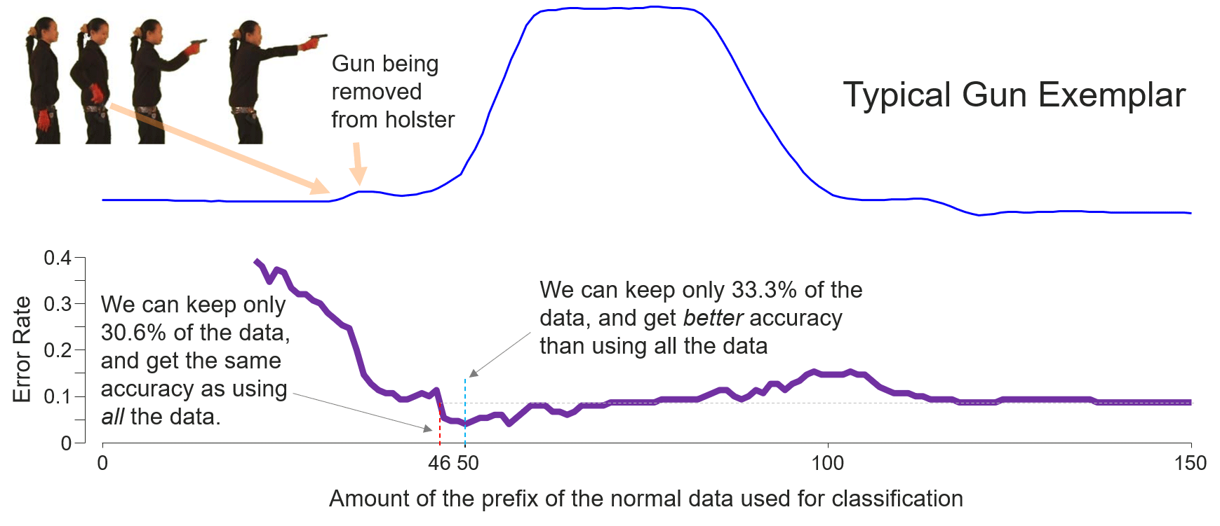
Fig. 9 (bottom) shows the reverse of the testing error-rate curve in the output.
Appendix B: 2nd Q&A
The results are presented in the presentation in section Slides.
To produce the results in the slides, we first run Java code
java -jar "/path/to/TEASERTester.jar" "GunPoint (TRAIN) + RandomWalk (TEST)" "/path/to/GunPoint_TRAIN.tsv" "/path/to/RandomWalk_TEST.tsv" "/path/to/output.json"
to generate the early predictions of each snapshot on every exemplars in the RandomWalk testing dataset.
The pre-compiled TEASERTester.jar can be found in section Code: Appendix B: 2nd Q&A;
GunPoint_TRAIN.tsv and RandomWalk_TEST.tsv can be found in section Data; /path/to/output.json
determines where results will be written.
Then we run MATLAB script TEASERResultPlotter.m (which can be found in section Code: Appendix B: 2nd Q&A):
TEASERResultPlotter("/path/to/output.json")
to draw the figures in the slides.
References
-
Z. Xing et al., “Early Classification on Time Series,” Knowledge and Information Systems, vol. 31, no. 1, pp. 105-127, 2012. ↩ ↩2 ↩3 ↩4
-
Z. Xing, “Zhengzheng Xing: PhD Research”. ↩ ↩2
-
Z. Xing et al., “Extracting Interpretable Features for Early Classification on Time Series,” in Proc. SIAM Intl. Conf. Data Mining, 2011, pp. 247-258. ↩ ↩2 ↩3 ↩4 ↩5
-
N. Parrish et al., “Classifying with Confidence from Incomplete Information,” J. Machine Learning Research, vol 14, no. 1, pp. 3561-3589, 2013. ↩ ↩2 ↩3 ↩4 ↩5
-
P. Schäfer and U. Leser, “TEASER: Early and Accurate Time Series Classification,” Data Mining and Knowledge Discovery, vol. 34, no. 5, pp. 1336-1362, 2020. ↩ ↩2